Getting Started

The aim of this section is to provide a short tutorial on how to getting started with the RBN toolbox. This tutorial is rather an overview over some basic features of the toolbox than an exhaustive explanation of all available functions. If you want to know what you can do with the RBN toolbox without reading the whole function reference, then this is your starting point. If you have doubts about what Random Boolean Networks are, then have a look at the RBN Overview. 

Initializing and visualizing the network

First of all, you have to decide what parameters your Random Boolean Network (RBN) will have. For reasons of clarity, we deal in this tutorial only with two parameters: N, the number of nodes in the network and K, the number of incoming connections per node.
These parameters remain generally constant over time, but there are also cases where one wants to change the network's topology after initialization. For this case, please consult the function reference.

There are a handful of functions that can be called to set up a Random Boolean Network. However, if one deals with a "standard" situation where only the parameters N and K are specified, then the easiest way to create the corresponding RBN is to use the bsn() function (Build and Show Network). In fact, this function calls all the basic initializing functions with some standard parameters and also calls a function to visualize the network's topology (displayTopology()). For example let's create a network with N = 8 and K = 2. At the Matlab command line type:

>> [node, conn, rule] = bsn(8,2,'arrow');

The variables node, conn and rule are matrices and contain information about node states, the logic transition rules associated to the nodes and the connections between the nodes. These three matrices are necessary and sufficient to represent the whole network and are therefore at the core of each session with the RBN toolbox. For details about internal representation of the network and these three matrices, have a look at the Matrix Representation section.

Matlab not only creates the matrices node, conn and rule, but also opens a new figure window displaying the network's topology.

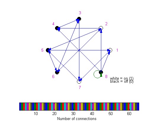
All nodes lie on an immaginary circle and are represented as small circles colored in black or white, according to their node state (zero or one). The colours of the directed connections represent the number of connections between two nodes, which can be determined by inspection of the Matlab color bar.

Calculating and visualizing the network's evolution

Now, we want to evolve our network over, let's say, 20 discrete time-steps and display the evolution. In order to do that, we just have to call the displayEvolution() function with the desired update scheme. There are a lot of different update schemes that are classified by their degree of synchronicity and determinism. For a description of all update modes consult the RBN Overview section. Here we choose for example the "Deterministic Generalized Asynchronous RBN" update mode (DGARBN). 

>> [node, tsm] = displayEvolution(node,20,'DGARBN');

node now contains information about all nodes at the end of the evolution, that is after time-step number 20. tsm is a time-state-matrix that contains all states of the nodes over the evolution time of 20 time-steps. The displayEvolution() function implicitly visualizes the time-state matrix:

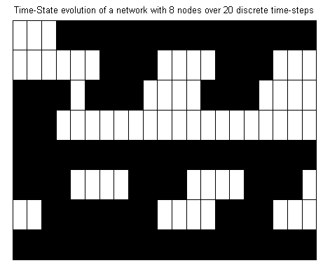
The x-axis corresponds to discrete time steps and the y-axis to the nodes. So in our case the time-state matrix is represented as a grid with 8x21 cells. The first column corresponds to the initial state of the network, the second column to the network's state after one time-step, etc. 
As the displayEvolution() function returns all information of the network at the end of the "DGARBN"-evolution, it is possible to take these node-states as initial values for an other evolution, let's say, in "Classical RBN" update mode. (CRBN)

>> [node, tsm] = displayEvolution(node,20,'CRBN');

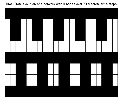
Finding the attractor

Obviously, after some time-steps our time-state matrix starts to exhibit some regular structure. To find the attractor, its length and the states in it, call the findAttractor() function.

>> [attrLength, attrStates] = findAttractor(node,tsm);

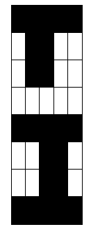
The variables attrLength and attrStates now contain the length of the attractor and all states in the attractor, respectively. By plotting the attrStates matrix, we find the attractor of our network, which is a sample of the evolution calculated before.

>> displayTimeStateMatrix(attrStates);

Visualizing node statistics

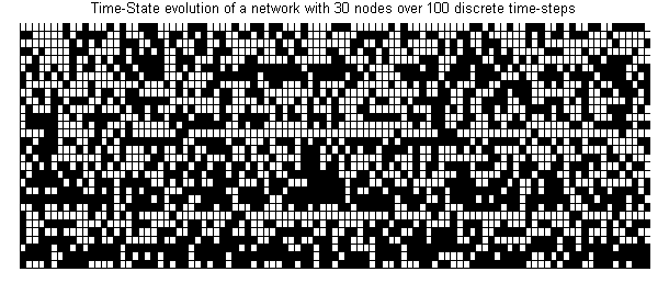
In this simple example, it is easy to keep an overview of the dynamics of the network. Yet, if a network with 30 nodes and 5 incoming connections per node is being evolved over 100 discrete time-steps in "CRBN" update mode, it may be useful to use some statistics.
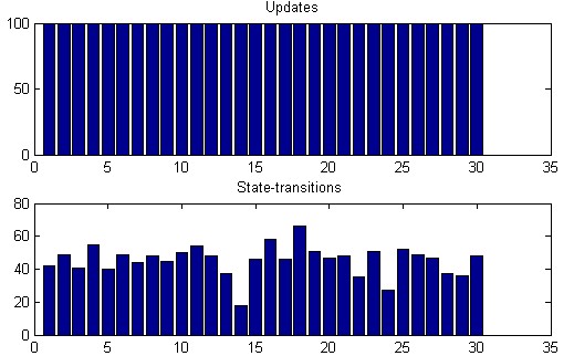
The displayNodeStats() function provides histogramms summing up the dynamics of the network.

>> [node2, conn2, rule2] = bsn(30,5,'arrow');
>> [node2, tsm2] = displayEvolution(node2,100,'CRBN');
>> displayNodeStats(node2, tsm2);

The corresponding node-statistics show the number of updates of each node and the effective number of transitions of each node. As the evolution has taken place in "CRBN" update-mode, it is clear that each node has been updated at each time-step.