|
Matrix Representation
This
section describes the internal representation of a Random Boolean
Network in the RBN Toolbox. In fact, there is one single
structure-array where all the information about nodes, connections
and logic transition rules is stored. This structure-array is
initialized by means of two matrices, which allows full control over
connections and rules.
The Connection-Matrix
The connection-matrix describes all connections in
the network. A network with N nodes has a connection-matrix of
size N x N, where an entry at (i,j) defines the number of
connections from node i to node j. Allowed entries for the
connection-matrix are positive integers including zero. However,
the maximum number of incoming connections per node is limited by
N, that is, the sum of all entries in a column must be smaller or
equal to N.
Example:
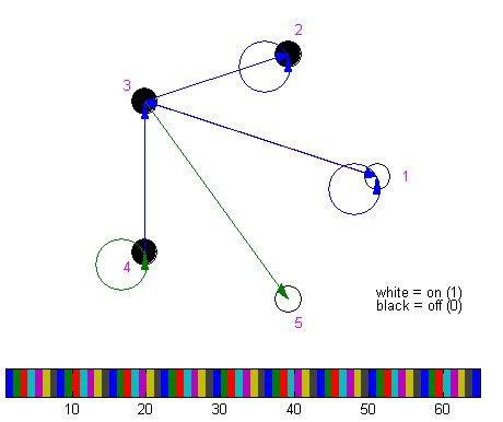
The corresponding network to the connection-matrix,
conn =
     1     0     1     0     0
     0     1     0     0     0
     1     1     0     0     2
     0     0     1     2     0
     0     0     0     0     0
would be:

Note, that the number of incoming connections in
this example is K=2, so the sum of all entries in a column is
always K. The sum of all entries in a row, however, can be zero or
any positive integer.
The
Rules-Matrix
The rules-matrix defines the
logic transition rules for each node in the network. For a network
with N nodes and K incoming connections per node the rules-matrix
has size
2^K x N. As each node n (n=1..N) has K incoming connections that
can transmit exactly two values, namely zero or one (off/on),
there are 2^K possible vectors as entry for a node. To each of
this vectors the node has to associate a binary output.
So, the entry at (i,j) in the rules-matrix defines the binary
output of node j to an input vector with value i. The value i of
an input vector is obtained by simply tranforming the sequence of
binary digits that correspond to values on the incoming
connections into a decimal integer. As in Matlab matrix indices always
start at 1 (and not at 0 as in a lot of other programming
languages), we have to add 1 to the integer number.
Example:
The following rules-matrix corresponds to a network with N=5 and
K=2. So there will be 2^K = 4 rows and 5 columns.
rule =
     0     0     1     0     1
     0     0     1     0     0
     1     1     0     1     0
     1     0     0     0     1
The logic transition rules
for node 2 are:
| Value on incoming
connection 1 |
Value on incoming
connection 2 |
State/Output |
| 0 |
0 |
0 |
| 0 |
1 |
0 |
| 1 |
0 |
1 |
| 1 |
1 |
0 |
The
Node-Structure-Array
The node-structure array is
at the core of each operation on a RBN. It contains all the
necessary information for displaying, evolving and changing the
network.
A network with N nodes has a node-structure-array that contains N
elements, each of them being a structure with the following
elements:
| Structure field |
Description |
| node.state |
Actual State (0 or 1) |
| node.nextState |
Next State (0 or 1) |
| node.nbUpdates |
Number of updates on this node |
| node.input |
Vector of indices to the incoming nodes |
| node.output |
Vector of indices to the outgoing nodes |
| node.p |
Update parameter p |
| node.q |
Update parameter q |
| node.lineNumber |
State-input-vector in decimal representation
= LUT (Look-Up-Table) rownumber |
| node.rule |
Vector containing transition logic rule for this node |
The fields node.input, node.output and node.rule contain
information that is identical to the information available in the
connection-matrix and rules-matrix. In fact, after the
node-structure-array has been initialized with these two matrices,
the connection-matrix and the rules-matrix are not used anymore.
This approach has been chosen because Matlab doesn't support
function parameter passing by reference. So instead of always
passing three matrices, it is now possible to deal with one
single, compact matrix, which is the node-structure array.
Nevertheless, as it might be convenient to define the connections
and rules in the network by means of matrices (as described
above), it is always possible to (re-)initialize the
node-structure-array with matrices using the functions
assocRules() and assocNeighbours().
|